Meta-Analytics for Soccer

r
soccer
To what extent does a state differentiate between players? How much does the stat’s value change over time?
Author

Tony ElHabr

Published

September 8, 2023

Introduction

This blog post demonstrates how to calculate the discrimination and stability “meta-metrics” proposed by Franks et al. (2017) for an array of soccer stats. Before the computations (“Inference”), I start by defining these meta-metrics (“Methods”), although I gloss over a lot of details for the sake of brevity. At the end, in “Results and Discussion”, I briefly discuss how my results compare to those for Franks et al., who analyzed basketball and hockey stats.

Background

In the realm of sports, data analysis has grown significantly, introducing numerous metrics to guide coaching, management, and, of course, fans. However, this proliferation has also led to confusion, with overlapping and sometimes conflicting metrics. To address this, Franks et al.1 propose three “meta-metrics” to help determine which metrics offer unique and dependable information for decision-makers.

By examining sources of variation in sports metrics (e.g. intrinsic player skill), Franks et al. introduce three meta-metrics to assess player performance stats:

  • discrimination: How good is the metric at telling players apart?
  • stability: How likely is it that a player maintains the same performance for the metric in the next season?
  • independence: Does the stat tell us something different about players that other stats don’t tell us?

Methods

Warning

I skip over a lot of details from Frank et al.’s paper here. I’d encourage an interested reader to review the original paper.

Discrimination

Simplifying the formulation of Franks et al., let’s define discrimination as follows:

\[ 1 - \frac{BV}{SV}. \tag{1}\]

\(BV\) is the average sampling variance of a metric after bootstrapping matches. (This variance measure is unique in that it involves resampling, while the others are simply calculated on the observed data.) \(SV\) is the total variance of a metric between players in a given season.

Altogether, this equation describes the fraction of variance between players due to true differences in player ability. A value closer to 1 indicates a metric that can differentiate between players more precisely.

Stability

Again, simplifying the original equation from Franks et al., we define stability as so:

\[ 1 - \frac{WV - BV}{TV - BV}. \tag{2}\]

\(WV\) represents the average variance among seasons “within” a player, before accounting for sampling variance (\(BV\)). \(TV\) is the total variance of a metric over all seasons, before accounting for sampling variance.

On the whole, this equation represent the fraction of total variance that is due to within-player changes over time. A value closer to 1 indicates that the metric value for a given player is less likely to change from season to season.

Inference

Data

We’ll be using public data from FBref for the 2018/19 - 2022/23 seasons of the the Big 5 European soccer leagues.

Retrieve and wrangle data
library(dplyr)
library(tidyr)
library(purrr)
library(tibble)

load_fb_advanced_match_stats <- function(country, gender, tier, stat_type, team_or_player, season_end_year = NA) {
  
  url <- sprintf(
    'https://github.com/JaseZiv/worldfootballR_data/releases/download/fb_advanced_match_stats/%s_%s_%s_%s_%s_advanced_match_stats.rds',
    country,
    gender,
    tier,
    stat_type,
    team_or_player
  )
  readRDS(url(url))
}

possibly_load_fb_advanced_match_stats <- purrr::possibly(
  load_fb_advanced_match_stats, 
  otherwise = tibble::tibble(),
  quiet = TRUE
)

params <- tidyr::expand_grid(
  country = c('ENG', 'ESP', 'FRA', 'GER', 'ITA'),
  gender = 'M',
  tier = '1st',
  stat_type = 'summary',
  team_or_player = 'player'
) |> 
  as.list()

raw_player_match_stats <- purrr::pmap_dfr(
  params,
  possibly_load_fb_advanced_match_stats
) |> 
  dplyr::filter(
    ## stop at 2022/23 season
    Season_End_Year < 2024L,
    ## don't include keepers
    !grepl('GK', Pos)
  )

ALL_METRICS <- c(
  'goals' = 'Goals',
  'assists' = 'Assists',
  'shots' = 'Shots',
  'shots_on_target' = 'Shots on Target',
  'tackles' = 'Tackles',
  'interceptions' = 'Interceptions',
  'xg' = 'xG',
  'xa' = 'xA',
  'goals_xg_ratio' = 'Goals/xG',
  'carries' = 'Carries',
  'shot_conversion_rate' = 'Shots Conversion Rate',
  'pass_completion_rate' = 'Pass Completion Rate',
  'goals_p90' = 'Goals/90',
  'shots_p90' = 'Shots/90',
  'xg_p90' = 'xG/90'
)

safe_divide <- function(num, den) {
  ifelse(
    den == 0 | is.na(den),
    NA_real_,
    dplyr::coalesce(num / den, 0)
  )
}

coalesce_fraction <- purrr::compose(
  \(num, den) safe_divide(num, den),
  \(x) ifelse(x > 1, 1, x),
  \(x) ifelse(x < 0, 0, x),
  .dir = 'forward'
)

add_rate_and_p90_metric_columns <- function(df) {
  df |> 
    dplyr::mutate(
      ## Mark Noble with the epic 1 goal on 0 shots https://fbref.com/en/matches/b56fd899/Watford-West-Ham-United-December-28-2021-Premier-League
      shot_conversion_rate = coalesce_fraction(goals, shots),
      pass_completion_rate = coalesce_fraction(passes_completed, passes_attempted),
      goals_xg_ratio = safe_divide(goals, xg)
    ) |> 
    dplyr::mutate(
      dplyr::across(
        c(goals, shots, xg),
        list(
          p90 = \(.x) 90 * .x / minutes_played
        )
      )
    )
}

summarize_all_metric_columns <- function(df, ...) {
  matches_played <- df |> 
    dplyr::group_by(league, season, team, player) |>
    dplyr::filter(minutes_played > 0L) |> 
    dplyr::summarize(
      matches_played = dplyr::n_distinct(match_id)
    ) |> 
    dplyr::ungroup()
  
  df |> 
    dplyr::group_by(..., league, season, team, player) |> 
    dplyr::summarize(
      dplyr::across(
        c(minutes_played:dplyr::last_col()),
        sum
      )
    ) |> 
    dplyr::ungroup() |> 
    add_rate_and_p90_metric_columns() |> 
    dplyr::inner_join(
      matches_played,
      by = dplyr::join_by(league, season, team, player)
    ) |> 
    dplyr::relocate(
      matches_played,
      .before = minutes_played
    )
}


player_match_stats <- raw_player_match_stats |> 
  dplyr::transmute(
    league = sprintf('%s-%s-%s', Country, Gender, Tier),
    season = sprintf('%s/%s', Season_End_Year - 1, substr(Season_End_Year, 3, 4)),
    date = Match_Date,
    match_id = basename(dirname(MatchURL)),
    team = Team,
    player = Player,
    
    minutes_played = Min,
    
    goals = Gls, ## includes pks
    assists = Ast,
    shots = Sh, ## does not include pk attempts
    shots_on_target = SoT,
    tackles = Tkl,
    interceptions = Int,
    
    passes_completed = Cmp_Passes,
    passes_attempted = Att_Passes,
    carries = Carries_Carries,
    
    xg = xG_Expected,
    xa = xAG_Expected
  ) |> 
  add_rate_and_p90_metric_columns()

player_season_stats <- summarize_all_metric_columns(player_match_stats)

## Franks et al. used 250 min played for the NBA
## https://github.com/afranks86/meta-analytics/blob/1871d24762184afa69f29a2b5b348431e70b9b2b/basketballReliability.R#L60
MIN_MINUTES_PLAYED <- 270
eligible_player_season_stats <- player_season_stats |> 
  dplyr::filter(minutes_played >= MIN_MINUTES_PLAYED)

eligible_player_match_stats <- player_match_stats |> 
  dplyr::semi_join(
    eligible_player_season_stats,
    by = dplyr::join_by(league, season, team, player)
  ) |> 
  dplyr::arrange(league, season, team, player)

## drop players with 0s for any given metric across any season?
##   looks like they only did that for testing a 1-season evaluation:
##   https://github.com/afranks86/meta-analytics/blob/1871d24762184afa69f29a2b5b348431e70b9b2b/basketballReliability.R#L25
# eligible_player_season_stats |> 
#   pivot_metric_columns() |> 
#   group_by(league, team, player, metric) |> 
#   summarize(has_any_zero = any(value == 0)) |> 
#   ungroup() |> 
#   filter(has_any_zero)
After some light wrangling, the player-match data looks like this.

dplyr::glimpse(eligible_player_match_stats)
#> Rows: 271,416
#> Columns: 24
#> $ league               <chr> "ENG-M-1st", "ENG-M-1st", "ENG-M-1st", "ENG-M-…
#> $ season               <chr> "2018/19", "2018/19", "2018/19", "2018/19", "2…
#> $ date                 <chr> "2018-08-12", "2018-08-18", "2018-08-25", "201…
#> $ match_id             <chr> "478e9dab", "9b69882c", "0014076a", "c1503e09"…
#> $ team                 <chr> "Arsenal", "Arsenal", "Arsenal", "Arsenal", "A…
#> $ player               <chr> "Aaron Ramsey", "Aaron Ramsey", "Aaron Ramsey"…
#> $ minutes_played       <dbl> 53, 23, 90, 90, 79, 79, 62, 24, 11, 13, 18, 16…
#> $ goals                <dbl> 0, 0, 0, 0, 0, 0, 0, 1, 0, 0, 0, 0, 0, 0, 0, 0…
#> $ assists              <dbl> 0, 0, 0, 0, 0, 2, 0, 1, 0, 0, 0, 1, 0, 2, 0, 0…
#> $ shots                <dbl> 1, 2, 2, 2, 0, 1, 0, 1, 0, 0, 0, 1, 0, 3, 1, 0…
#> $ shots_on_target      <dbl> 1, 1, 1, 2, 0, 1, 0, 1, 0, 0, 0, 1, 0, 0, 0, 0…
#> $ tackles              <dbl> 2, 0, 2, 1, 2, 0, 2, 0, 1, 0, 0, 0, 1, 2, 1, 0…
#> $ interceptions        <dbl> 0, 0, 1, 2, 0, 0, 0, 0, 0, 0, 0, 1, 0, 0, 0, 0…
#> $ passes_completed     <dbl> 9, 6, 48, 51, 49, 26, 16, 16, 13, 5, 11, 7, 8,…
#> $ passes_attempted     <dbl> 13, 9, 61, 66, 58, 31, 20, 21, 15, 7, 12, 10, …
#> $ carries              <dbl> 5, 7, 41, 49, 43, 27, 21, 16, 11, 8, 11, 7, 7,…
#> $ xg                   <dbl> 0.0, 0.1, 0.1, 0.1, 0.0, 0.0, 0.0, 0.1, 0.0, 0…
#> $ xa                   <dbl> 0.1, 0.0, 0.2, 0.2, 0.1, 0.4, 0.0, 0.1, 0.0, 0…
#> $ shot_conversion_rate <dbl> 0, 0, 0, 0, NA, 0, NA, 1, NA, NA, NA, 0, NA, 0…
#> $ pass_completion_rate <dbl> 0.6923077, 0.6666667, 0.7868852, 0.7727273, 0.…
#> $ goals_xg_ratio       <dbl> NA, 0.000000, 0.000000, 0.000000, NA, NA, NA, …
#> $ goals_p90            <dbl> 0.000000, 0.000000, 0.000000, 0.000000, 0.0000…
#> $ shots_p90            <dbl> 1.698113, 7.826087, 2.000000, 2.000000, 0.0000…
#> $ xg_p90               <dbl> 0.0000000, 0.3913043, 0.1000000, 0.1000000, 0.…

There are a lot more stats we could pull in, but I’ve opted for a relatively small set of 15 stats2:

  • “Un-adjusted” (i.e. not normalized for the number of minutes played) counting stats: goals, assists, shots, shots on target, tackles, interceptions, and carries
  • Un-adjusted “advanced” stats: expected goals (xG), expected assists (xA), and goals/xG ratio
  • Rate metrics: pass completion rate and shot conversion rate (i.e. goals divided by shots)
  • “Per 90” versions of other stats: goals/90, shots/90, and xG/90

Now we can start to calculate the meta-metrics.

Discrimination

We’ll begin with the discrimination meta-metric, which means we’ll need to calculate “bootstrap variance”, \(BV\), and, “seasonal variance”, \(SV\), as shown in Equation 1.

Starting with the former, we resample player matches within teams, with replacement.

Bootstrap observed player-seasons
resample_stats <- function(player_match_stats) {
  
  match_ids <- player_match_stats |>
    dplyr::distinct(league, season, team, date, match_id) |> 
    dplyr::arrange(league, season, team, date)
  
  ## can't just specify to resample 38 matches per team since different leagues 
  ## have different season lengths (Bundesliga)
  resampled_match_ids <- match_ids |> 
    dplyr::select(league, season, team, match_id) |> 
    dplyr::group_by(league, season, team) |> 
    dplyr::summarize(
      match_id = list(match_id)
    ) |> 
    dplyr::ungroup() |> 
    dplyr::mutate(
      match_id = purrr::map(
        match_id,
        \(.x) {
          sample(.x, size = length(.x), replace = TRUE)
        })
    ) |> 
    tidyr::unnest(match_id)
  
  resampled_match_ids |> 
    dplyr::inner_join(
      player_match_stats,
      by = dplyr::join_by(league, season, team, match_id),
      relationship = 'many-to-many'
    )
}

## Franks et al. used 20 bootstrap replicates
## https://github.com/afranks86/meta-analytics/blob/1871d24762184afa69f29a2b5b348431e70b9b2b/basketballReliability.R#L70
N_BOOSTRAPS <- 20
set.seed(42)
resampled_player_match_stats <- purrr::map_dfr(
  rlang::set_names(1:N_BOOSTRAPS),
  \(...) {
    resample_stats(
      player_match_stats = eligible_player_match_stats
    )
  },
  .id = 'bootstrap_id'
) |> 
  dplyr::mutate(bootstrap_id = as.integer(bootstrap_id))

After we aggregate over the matches in each bootstrap to create player-season summaries per bootstrap, we get a data frame that looks like this.

Aggregate bootstraps
resampled_player_match_stats <- resampled_player_match_stats |> 
  ## Franks et al. did this
  ## https://github.com/afranks86/meta-analytics/blob/1871d24762184afa69f29a2b5b348431e70b9b2b/basketballReliability.R#L78
  dplyr::filter(minutes_played < (0.75 * MIN_MINUTES_PLAYED))

resampled_player_season_stats <- resampled_player_match_stats |> 
  summarize_all_metric_columns(bootstrap_id) |> 
  dplyr::arrange(bootstrap_id, league, season, team, player)
dplyr::glimpse(resampled_player_season_stats)
#> Rows: 234,172
#> Columns: 24
#> $ bootstrap_id         <int> 1, 1, 1, 1, 1, 1, 1, 1, 1, 1, 1, 1, 1, 1, 1, 1…
#> $ league               <chr> "ENG-M-1st", "ENG-M-1st", "ENG-M-1st", "ENG-M-…
#> $ season               <chr> "2018/19", "2018/19", "2018/19", "2018/19", "2…
#> $ team                 <chr> "Arsenal", "Arsenal", "Arsenal", "Arsenal", "A…
#> $ player               <chr> "Aaron Ramsey", "Ainsley Maitland-Niles", "Ale…
#> $ matches_played       <int> 28, 16, 35, 35, 29, 25, 19, 17, 34, 33, 24, 8,…
#> $ minutes_played       <dbl> 1349, 1053, 1714, 2767, 2213, 1357, 989, 1385,…
#> $ goals                <dbl> 2, 2, 3, 11, 4, 3, 0, 5, 0, 0, 7, 0, 2, 20, 0,…
#> $ assists              <dbl> 1, 1, 4, 8, 2, 5, 3, 0, 3, 0, 2, 0, 4, 4, 0, 5…
#> $ shots                <dbl> 28, 8, 31, 102, 24, 30, 7, 5, 21, 20, 14, 9, 7…
#> $ shots_on_target      <dbl> 9, 6, 15, 28, 11, 11, 4, 5, 1, 4, 9, 0, 6, 27,…
#> $ tackles              <dbl> 37, 28, 21, 35, 44, 17, 9, 21, 61, 35, 9, 21, …
#> $ interceptions        <dbl> 10, 17, 14, 19, 34, 9, 13, 36, 55, 23, 3, 0, 3…
#> $ passes_completed     <dbl> 733, 444, 619, 677, 1656, 552, 470, 832, 1269,…
#> $ passes_attempted     <dbl> 906, 561, 847, 933, 2059, 724, 580, 905, 1504,…
#> $ carries              <dbl> 630, 334, 724, 738, 1085, 454, 333, 602, 978, …
#> $ xg                   <dbl> 2.7, 1.6, 4.2, 11.0, 1.0, 3.9, 0.3, 1.9, 0.6, …
#> $ xa                   <dbl> 2.4, 0.9, 5.3, 3.6, 2.0, 4.8, 0.9, 0.5, 0.7, 0…
#> $ shot_conversion_rate <dbl> 0.07142857, 0.25000000, 0.09677419, 0.10784314…
#> $ pass_completion_rate <dbl> 0.8090508, 0.7914439, 0.7308146, 0.7256163, 0.…
#> $ goals_xg_ratio       <dbl> 0.7407407, 1.2500000, 0.7142857, 1.0000000, 4.…
#> $ goals_p90            <dbl> 0.1334322, 0.1709402, 0.1575263, 0.3577882, 0.…
#> $ shots_p90            <dbl> 1.8680504, 0.6837607, 1.6277713, 3.3176726, 0.…
#> $ xg_p90               <dbl> 0.180133432, 0.136752137, 0.220536756, 0.35778…

Next, we calculate the variance across the player-season bootstraps, and then average the bootstrap variance over all player-seasons, grouping by season, to arrive at \(BV\). We end up with one variance value per season and metric.

Calculate average bootstrap variance, BV
pivot_metric_columns <- function(df) {
  df |> 
    dplyr::select(
      league,
      season,
      team,
      player,
      dplyr::any_of(names(ALL_METRICS))
    ) |> 
    tidyr::pivot_longer(
      -c(league, season, team, player),
      names_to = 'metric',
      values_to = 'value'
    )
}

resampled_player_season_variance <- resampled_player_season_stats |> 
  pivot_metric_columns() |> 
  dplyr::group_by(season, team, player, metric) |> 
  dplyr::summarize(
    bv = var(value, na.rm = TRUE)
  ) |> 
  dplyr::ungroup()

bv <- resampled_player_season_variance |> 
  dplyr::group_by(season, metric) |> 
  dplyr::summarize(
    bv = mean(bv, na.rm = TRUE)
  ) |> 
  dplyr::ungroup() |> 
  dplyr::arrange(season, metric)
bv
#> # A tibble: 90 × 3
#>    season  metric                        bv
#>    <chr>   <chr>                      <dbl>
#>  1 2017/18 assists                 1.64    
#>  2 2017/18 carries              7712.      
#>  3 2017/18 goals                   2.36    
#>  4 2017/18 goals_p90               0.0102  
#>  5 2017/18 goals_xg_ratio          1.40    
#>  6 2017/18 interceptions          33.4     
#>  7 2017/18 pass_completion_rate    0.000577
#>  8 2017/18 shot_conversion_rate    0.00604 
#>  9 2017/18 shots                  32.5     
#> 10 2017/18 shots_on_target         8.39 
#> # ℹ 80 more rows

Next, we move on to the “seasonal variance”, \(SV\). This is actually pretty trivial, as it’s just a direct call to stats::var on the observed player-season aggregates, grouping by season. Again, we end up with one row per season and metric.

Calculate seasonal variance, SV
pivoted_player_season_stats <- pivot_metric_columns(player_season_stats)

sv <- pivoted_player_season_stats |>
  dplyr::group_by(season, metric) |> 
  dplyr::summarize(
    sv = var(value, na.rm = TRUE)
  ) |> 
  dplyr::ungroup() |> 
  dplyr::arrange(season, metric)
sv
#> # A tibble: 90 × 3
#>    season  metric                         sv
#>    <chr>   <chr>                       <dbl>
#>  1 2017/18 assists                   4.33   
#>  2 2017/18 carries              153542.     
#>  3 2017/18 goals                    12.4    
#>  4 2017/18 goals_p90                 0.302  
#>  5 2017/18 goals_xg_ratio            2.15   
#>  6 2017/18 interceptions           319.     
#>  7 2017/18 pass_completion_rate      0.00948
#>  8 2017/18 shot_conversion_rate      0.0128 
#>  9 2017/18 shots                   480.     
#> 10 2017/18 shots_on_target          73.4    
#> # ℹ 80 more rows

Finally, we bring \(BV\) and \(SV\) together to calculate discrimination by season.

Calculate discrimination
discrimination <- bv |> 
  dplyr::inner_join(
    sv,
    by = dplyr::join_by(season, metric)
  ) |> 
  dplyr::mutate(
    discrimination = 1 - bv / sv
  ) |> 
  dplyr::arrange(season, metric)
discrimination
#> # A tibble: 90 × 5
#>    season  metric                        bv           sv discrimination
#>    <chr>   <chr>                      <dbl>        <dbl>          <dbl>
#>  1 2017/18 assists                 1.64          4.33             0.621
#>  2 2017/18 carries              7712.       153542.               0.950
#>  3 2017/18 goals                   2.36         12.4              0.810
#>  4 2017/18 goals_p90               0.0102        0.302            0.966
#>  5 2017/18 goals_xg_ratio          1.40          2.15             0.348
#>  6 2017/18 interceptions          33.4         319.               0.895
#>  7 2017/18 pass_completion_rate    0.000577      0.00948          0.939
#>  8 2017/18 shot_conversion_rate    0.00604       0.0128           0.527
#>  9 2017/18 shots                  32.5         480.               0.932
#> 10 2017/18 shots_on_target         8.39         73.4              0.886
#> # ℹ 80 more rows

For the sake of making discrimination directly comparable to stability (which is only calculated per metric, not per metric and season), we can average the discrimination values over all seasons.

Average discrimination
average_discrimination <- discrimination |> 
  dplyr::group_by(metric) |> 
  dplyr::summarize(
    discrimination = mean(discrimination)
  ) |> 
  dplyr::arrange(metric)
average_discrimination
#> # A tibble: 15 × 2
#>    metric               discrimination
#>    <chr>                         <dbl>
#>  1 assists                       0.600
#>  2 carries                       0.951
#>  3 goals                         0.792
#>  4 goals_p90                     0.830
#>  5 goals_xg_ratio                0.181
#>  6 interceptions                 0.889
#>  7 pass_completion_rate          0.950
#>  8 shot_conversion_rate          0.507
#>  9 shots                         0.926
#> 10 shots_on_target               0.875
#> 11 shots_p90                     0.956
#> 12 tackles                       0.895
#> 13 xa                            0.830
#> 14 xg                            0.898
#> 15 xg_p90                        0.929

Stability

For stability, we need to calculate “within”-player variance, \(WV\), and “total variance”, \(TV\), as shown in Equation 2.

For \(WV\), we start by grouping on the on everything but the metric values and season variable in our data frame for observed player-season stats, and calculate variance with var(). Then we average the variance across all players with mean().

Calculate within-player variance, WV
within_player_variance <- pivoted_player_season_stats |> 
  ## should check for players with the same name
  dplyr::group_by(league, team, player, metric) |>
  dplyr::summarize(
    seasons_played = dplyr::n(),
    wv = var(value, na.rm = TRUE)
  ) |> 
  dplyr::ungroup()

wv <- within_player_variance |>
  ## Franks et al. don't have something quite like this, where they filter for
  ##   a minimum number of seasons played. I think they didn't find it necessary
  ##   after dropping player who have ever had zeros, and because they were working
  ##   with 20 seasons of NBA data. (I'm working with 6.)
  dplyr::filter(
    seasons_played >= 3L
  ) |> 
  dplyr::group_by(metric) |> 
  dplyr::summarize(
    wv = mean(wv, na.rm = TRUE)
  ) |> 
  dplyr::ungroup() |> 
  dplyr::arrange(metric)
wv
#> # A tibble: 15 × 2
#>    metric                        wv
#>    <chr>                      <dbl>
#>  1 assists                  2.71   
#>  2 carries              77143.     
#>  3 goals                    5.75   
#>  4 goals_p90                0.0269 
#>  5 goals_xg_ratio           1.45   
#>  6 interceptions          122.     
#>  7 pass_completion_rate     0.00339
#>  8 shot_conversion_rate     0.0103 
#>  9 shots                  183.     
#> 10 shots_on_target         29.1    
#> 11 shots_p90                0.821  
#> 12 tackles                239.     
#> 13 xa                       1.57   
#> 14 xg                       3.71   
#> 15 xg_p90                   0.0141

To finish our variance calculations, we calculate “total variance”, \(TV\). This is the most straightforward of them all, as it involves just a call to var() for each metric on the observed player-season stats.

Calculate total variance, TV
tv <- pivoted_player_season_stats |> 
  dplyr::group_by(metric) |>
  dplyr::summarize(
    tv = var(value, na.rm = TRUE)
  ) |> 
  dplyr::ungroup() |> 
  dplyr::arrange(metric)
tv
#> # A tibble: 15 × 2
#>    metric                        tv
#>    <chr>                      <dbl>
#>  1 assists                   4.16  
#>  2 carries              161078.    
#>  3 goals                    11.5   
#>  4 goals_p90                 0.0925
#>  5 goals_xg_ratio            1.67  
#>  6 interceptions           252.    
#>  7 pass_completion_rate      0.0119
#>  8 shot_conversion_rate      0.0136
#>  9 shots                   427.    
#> 10 shots_on_target          65.2   
#> 11 shots_p90                 4.76  
#> 12 tackles                 460.    
#> 13 xa                        3.15  
#> 14 xg                        9.27  
#> 15 xg_p90                    0.0729

We bring \(BV\), \(WV\) and \(TV\) together to calculate stability.

Calculate stability
average_bv <- bv |> 
  dplyr::group_by(metric) |> 
  dplyr::summarize(
    bv = mean(bv)
  ) |> 
  dplyr::ungroup()

stability <- average_bv |> 
  dplyr::inner_join(
    tv,
    by = dplyr::join_by(metric)
  ) |>
  dplyr::inner_join(
    wv,
    by = dplyr::join_by(metric)
  ) |> 
  dplyr::mutate(
    stability = 1 - (wv - bv) / (tv - bv)
  ) |> 
  dplyr::arrange(metric)
stability
#> # A tibble: 15 × 5
#>    metric                        bv          tv          wv stability
#>    <chr>                      <dbl>       <dbl>       <dbl>     <dbl>
#>  1 assists                 1.66          4.16       2.71        0.580
#>  2 carries              7808.       161078.     77143.          0.548
#>  3 goals                   2.38         11.5        5.75        0.629
#>  4 goals_p90               0.0105        0.0925     0.0269      0.799
#>  5 goals_xg_ratio          1.35          1.67       1.45        0.696
#>  6 interceptions          27.8         252.       122.          0.577
#>  7 pass_completion_rate    0.000582      0.0119     0.00339     0.752
#>  8 shot_conversion_rate    0.00670       0.0136     0.0103      0.487
#>  9 shots                  31.7         427.       183.          0.618
#> 10 shots_on_target         8.17         65.2       29.1         0.634
#> 11 shots_p90               0.118         4.76       0.821       0.849
#> 12 tackles                48.3         460.       239.          0.537
#> 13 xa                      0.538         3.15       1.57        0.607
#> 14 xg                      0.944         9.27       3.71        0.668
#> 15 xg_p90                  0.00397       0.0729     0.0141      0.853

Results and Discussion

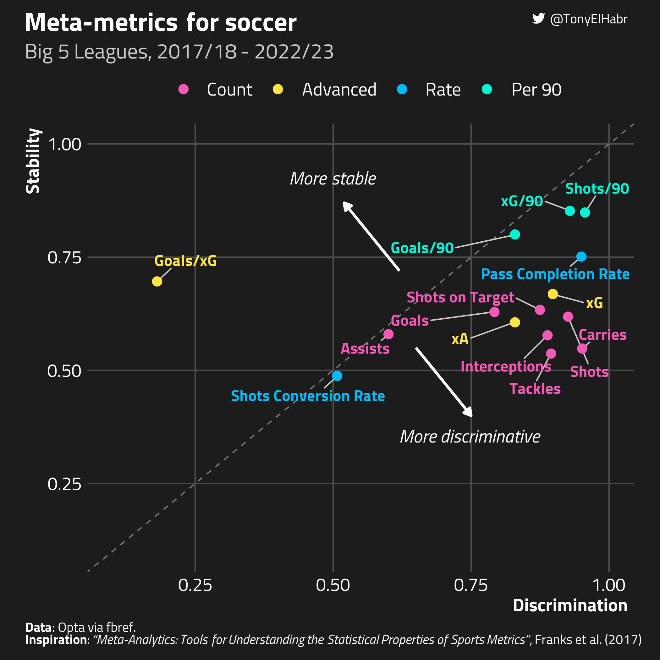
Let’s make a scatter plot of the discrimination and stability of our metrics, akin to the plots made by Franks et al.

We can make the following observations:

  • Un-adjusted volume (i.e. “count” in the plot) statistics based on total playing time–like shots, tackles, and interceptions–tend to be highly discriminative, but not quite as stable. This makes sense—such statistics have large between-player variance—think about the number of shots that a central defender takes compared to a striker. When aggregated for each player throughout a season, they provide a strong signal for different player types, i.e. positions. Indeed, Franks et al. found the same for NBA and NHL statistics.

  • Advanced stats like xG and xA also prove to be more discriminative than stable.

  • The other advanced stat, goals/xG ratio, stands out. It’s the only metric that is significantly more stable than discriminative. Although I haven’t looked into this extensively or given it much more than a few moments of thought, I believe this is because most players do not score goals in individual matches, but often accumulate some non-zero xG via shots. Thus, Goals/xG can be zero very frequently, meaning that it would be hard to differentiate players just on this ratio. And, because the ratio is often zero, it is found to be stable.

  • Shot conversion rate seems to be the center of the universe, having nearly equal discrimination and stability, both at around 0.5.

  • The per 90 metrics show higher stability than all other stats evaluated. This speaks to the between-player noise-minimizing benefits of comparing players on an equal-minute basis. Their stability is much closer to their discriminative power than most other other metrics.

Conclusion

We’ve replicated the ideas of a commonly cited sports analytics paper3, applying them to the beautiful game of soccer. While this blog post was more about replication than insights, we’ve confirmed that the key observations regarding the meta-metric properties of volume and rate statistics also apply soccer.

  • Discrimination can be used to distinguish between players for a given season. Volume measures like shots and tackles should implicitly provide some indication of player positions and roles. (After all, we wouldn’t expect a striker to be making more tackles than a defender.)
  • Stability represents how much a metric can vary over time. Intuitively, stats that adjust for playing time (i.e. “per 90”) show less fluctuations from season to season.
No matching items

Footnotes

  1. If it means anything, the Meta-analytics paper has 40 citations at the time of writing, suggesting it has had a non-trivial influence on subsequent sports analytics research.↩︎

  2. This isn’t meant to be an explainer of what these stats are or why they were chosen. Nonetheless, it’s worth pointing out the different types of stats, as it is relevant to the calculation relationship between discrimination and stability, as we shall see.↩︎

  3. The fact that they’ve published their code made the replication much less of a daunting task, so huge kudos to the authors. (Note that there were a few tweaks that I needed to make to get all of the code working properly with R >4.0.)↩︎